miWorkbench: Interpretability Workbench
The research workbench of miStudio. miWorkbench trains sparse autoencoders, labels and clusters what they find, discovers and causally tests circuits, reads the model layer by layer with J-Lens, and trains probe monitors that come with honest evidence about how well they work. An agent can drive all of it through a Model Context Protocol server, with a person approving anything that uses a graphics card.
Part of miStudio, and fully usable on its own.
miWorkbench (formerly miStudio) is where the suite looks inside a model. The work of mechanistic interpretability (training sparse autoencoders, finding features, labeling them, testing what they do, and turning what holds up into something usable) is usually spread across notebooks and one-off scripts. miWorkbench puts it in one database-backed application, so every run, extraction, label and test is recorded with the exact settings that produced it and can be found again later.
It runs any model that Hugging Face Transformers can load, without architecture-specific code, and spreads its work across however many graphics processing units (GPUs) the machine has, pinning each job to a card by its identifier.
The sparse-autoencoder pipeline
A sparse autoencoder (SAE) decomposes a layer’s dense activations into a much larger set of sparsely active features, many of which correspond to recognizable concepts (Cunningham et al., 2023). miWorkbench covers the full pipeline:
- Data and models from Hugging Face, with optional 4-bit or 8-bit loading and automatic discovery of every layer and hook point.
- SAE training with six architectures, including a rectified linear unit (ReLU) with an L1 penalty, JumpReLU (Rajamanoharan et al., 2024), TopK (Gao et al., 2024) and transcoders, with live loss and sparsity curves. Pretrained SAEs from Hugging Face can be used instead.
- Feature extraction, which records the top activating examples for each feature.
- Labeling by any large language model (LLM) behind an OpenAI-compatible endpoint, including a model served by miServer.
- Export to Hugging Face and Neuronpedia.
Labeling at scale, and knowing what is left
Labeling a 53,000-feature extraction takes days of GPU time and gets interrupted. miWorkbench records the outcome of every labeling attempt separately from the label. Before it did, a failed attempt was stored as a placeholder label, and 16,824 failures across our own extractions looked like finished work.
Each extraction now shows a coverage strip (adjudicated · failed · not attempted) with the failures grouped by cause. A feature the judge honestly found uninterpretable counts as adjudicated: that is a result, not a gap. Retrying 14,560 failures would take about thirty-two GPU-hours, so miWorkbench offers a twenty-feature sample first, which takes about three minutes. On one extraction the sample came back 20 of 20, but 18 were honest refusals, which turned “recover 14,560 labels” into “gain about 1,450 labels and close about 13,100 features for good”. Resume all then sweeps the remaining batches unattended under a GPU-hour ceiling stated before anything starts. Each label also records which judge produced it, fingerprinted by prompt and model, so improving a prompt marks exactly the affected labels stale.
Feature clusters
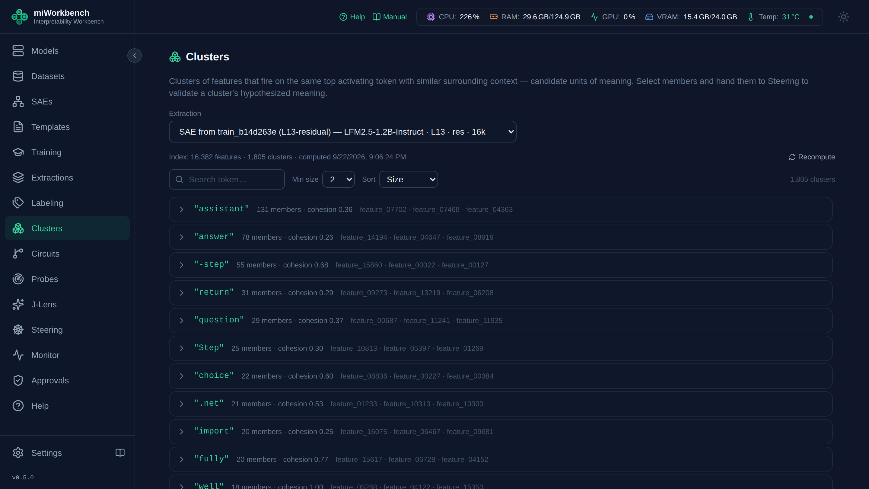
One extraction can surface tens of thousands of features, with related concepts scattered among them. The Feature Groups panel gathers features that share meaning and scores each group’s cohesion. A group’s hypothesized meaning can then be tested by steering its members together, and a tuned cluster exports as a mistudio.cluster-definition/v1 document that miServer can serve.
Circuits, graded by an evidence ladder
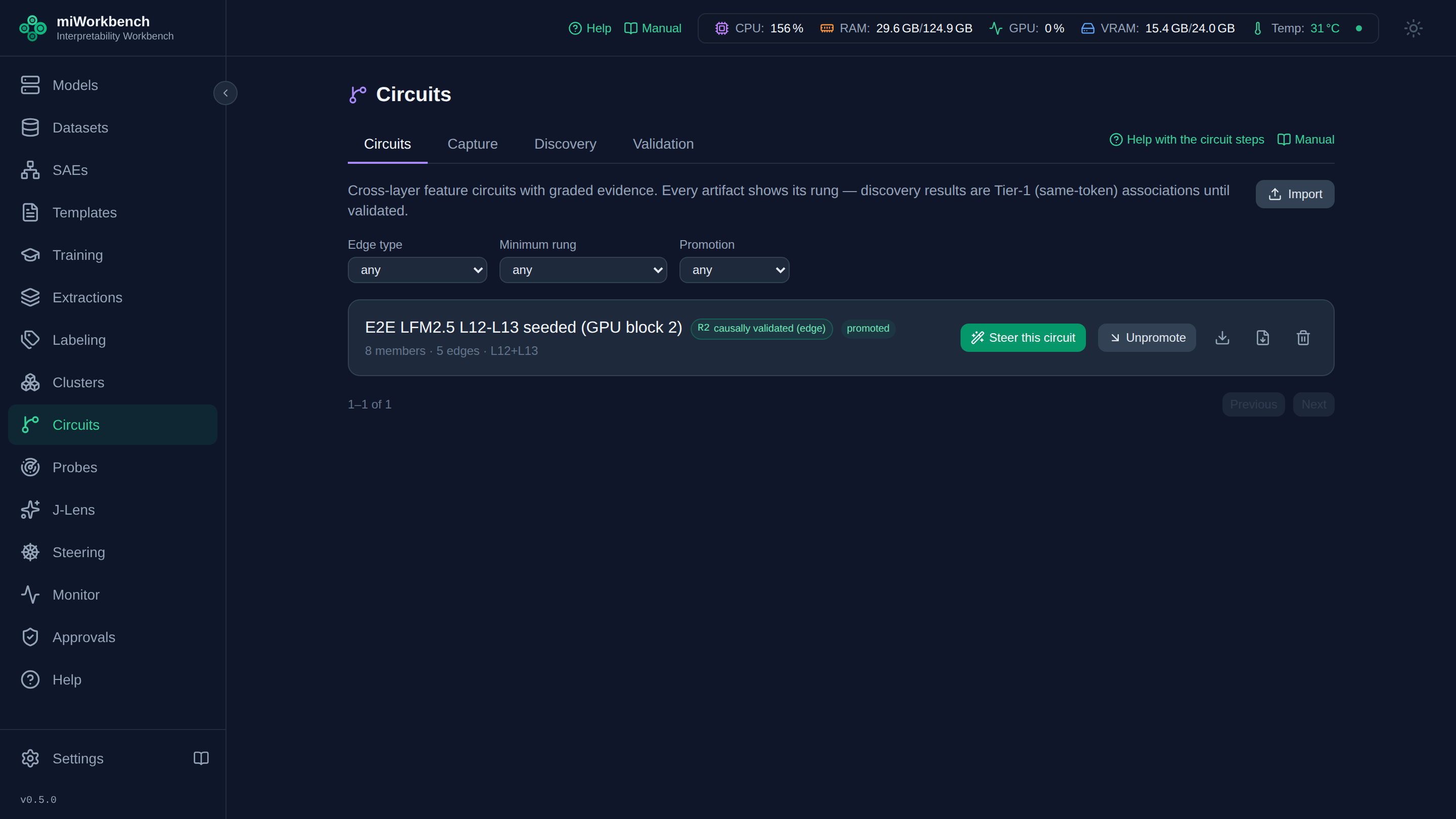
miWorkbench discovers circuits: how a feature at one layer drives a feature at a later one. Discovery captures activations at several layers and mines candidate edges statistically, with pointwise mutual information ranking, a null model, false-discovery-rate control (Benjamini and Hochberg, 1995) and held-out replication. It then adds gradient attribution as a second, independent signal, and finally tests edges by intervention: suppress the upstream feature and measure what happens downstream.
Discovery is not proof, so every edge and circuit carries a rung:
| Rung | Name | What earned it |
|---|---|---|
| 0 | mined | A statistical association, disclosed as one |
| 1 | attribution-supported | Gradient attribution agrees in sign and size; still not causal |
| 2 | causally validated | An intervention shows a real effect beyond a matched null |
| 3 | faithfulness-tested | The circuit’s members are shown to be necessary and sufficient for the behavior |
A circuit is only as strong as its weakest edge. The word “causal” never appears below rung 2, and the wording comes from the server so no screen can overstate it. A failed test is kept as history rather than hidden. Validated circuits export as mistudio.circuit-definition/v1, with a calibrated strength, for miServer to serve; miServer refuses one below rung 2 unless someone records that they accept the risk.
J-Lens: what the model is poised to say
J-Lens shows, for every layer and token position, the tokens the model is poised to produce at that point. The basic readout is the logit lens, which projects the residual stream through the model’s own output layer and works on any loaded model. A second lens, the Jacobian lens, uses a fitted per-layer matrix that recovers content earlier in the stack. miWorkbench fits one for the model at hand and checks it against a validation gate before it is used. Until a fitted lens exists, the Jacobian views are disabled with the reason stated, and miWorkbench never shows logit-lens data under a Jacobian label.
Steering
Steering adds a scaled feature direction to the model’s activations during generation. miWorkbench’s steering is built for comparison rather than a single slider: sweep one feature across strengths against the same prompt, compare many features side by side, or blend several into one generation. A frequency-derived baseline suggests a starting strength for each feature.
Probe monitors, with honest evidence
A probe monitor is a small linear readout of one layer’s activations, in the tradition of linear classifier probes (Alain and Bengio, 2016). It answers one question: is this behavior present in what the model is processing? A probe costs a dot product per forward pass, where a judge model costs a whole forward pass of its own. That trade is only worth making if you know what you are giving up, so most of this feature is measurement.
- Two kinds of probe. A dense probe reads the raw residual stream. A k-sparse probe reads an SAE’s features and gives one interpretable weight per feature.
- Pooling and layers. Each run sweeps layers and trains mean, max and attention pooling. It sets the threshold from known negatives at a target false-positive rate and reports bootstrapped confidence intervals.
- Judge baselines. A judge model can score the same evaluation rows so the probe’s numbers have something to be read against. Judges are driven by a judge-prompt library: versioned prompts, immutable once used, each tagged with the behavior it judges. Prompts can be added in the interface, over MCP, or by importing a miDataworks rubric, with no code change.
- Export. A probe exports as
mistudio.probe-definition/v1, with test vectors that let miServer prove it scores identically before it trusts a verdict.
Every probe carries its own rung, computed from what actually ran:
| Rung | Meaning |
|---|---|
| 0 | trained |
| 1 | detects on held-out data from the same distribution |
| 2 | detects on unseen tasks: an out-of-distribution set, with the confidence interval’s lower bound clearing chance |
| 3 | detects on unseen tasks, compared with a judge of the same behavior |
“Compared with” is deliberate. On miWorkbench’s reference run the judge won on all five evaluation sets, averaging 0.874 against the probe’s 0.794 area under the receiver operating characteristic curve (AUROC). A probe’s case on a small model is cost and latency, not accuracy, and the rung does not claim otherwise. The ladder also never calls a probe causal: causal language is earned only by intervention. For a probe that did well, see the personal-data walkthrough, along with the reasons not to over-read it.
Agent control through MCP
miWorkbench runs a Model Context Protocol (MCP) server with about 280 tools in 20 categories. It covers feature analysis, clustering, circuit discovery and validation, J-Lens, steering, labeling, probes and judge prompts. It also hosts the agent surface for its siblings: a miserver_* family that loads models, imports probes and circuits, steers and scores on a running miServer, and a dataworks_* family that reads and sends miDataworks datasets.
Agents can read, plan and analyze freely. Training or evaluating a probe, running a judge on miServer, and loading a model on miServer each file an approval request in a banner at the top of every panel. The agent re-calls with the approval’s identifier once a person approves, and a read-only approval-status tool lets it check first. A GPU preflight and a list of active jobs tell an agent whether a card is free before it asks for one. Results appear in the interface as they happen, so a person can pick up anything an agent started.
What miWorkbench exchanges with its siblings
| With | Direction | What |
|---|---|---|
| miDataworks | in | Probe datasets with their midataworks.dataset-version/v1 manifests, registered as training, evaluation and calibration views; rubrics as judge prompts |
| miDataworks | out | Probe results and evaluation scores, read back by miDataworks |
| miServer | out | Probe, circuit and cluster definitions |
| miServer | uses | Its OpenAI-compatible endpoint, as a labeler or a judge |
Each integration is detected at runtime. Without miDataworks, datasets come straight from Hugging Face; without miServer, labeling and judging use any OpenAI-compatible endpoint.
Being built
As part of the suite’s behavior-monitoring work, miWorkbench is gaining a behavior catalogue, a single record of each behavior’s definition, data, probes, judge prompts and operating point, and judge spot-checks of live miServer sessions that report how often probe and judge agree. The catalogue’s data model has landed; its screens and the spot-checks are in progress. See miStudio for the whole picture.
Explore miWorkbench
- Manual: docs-miworkbench.hitsai.net, including probe monitors, the evidence ladder, J-Lens and the MCP server
- Overview video: miWorkbench overview on YouTube
- Videos: YouTube channel
- Source code: github.com/hitsainet/miWorkbench (Apache 2.0)
- The rest of the suite: miStudio · miServer · miDataworks · miForge